HELP
BIPSPI can be employed to predict partner-specific protein-protein interfaces using as input two sequences, two structural models or one sequence and one structural model.
Additionally, it can be employed to launch PatchDock, a light protein-protein docking algorithm, using BIPSPI predictions as restrains.
BIPSPI predictions can be launched using "PREDICT binding sites" option (Figure 1, red box)
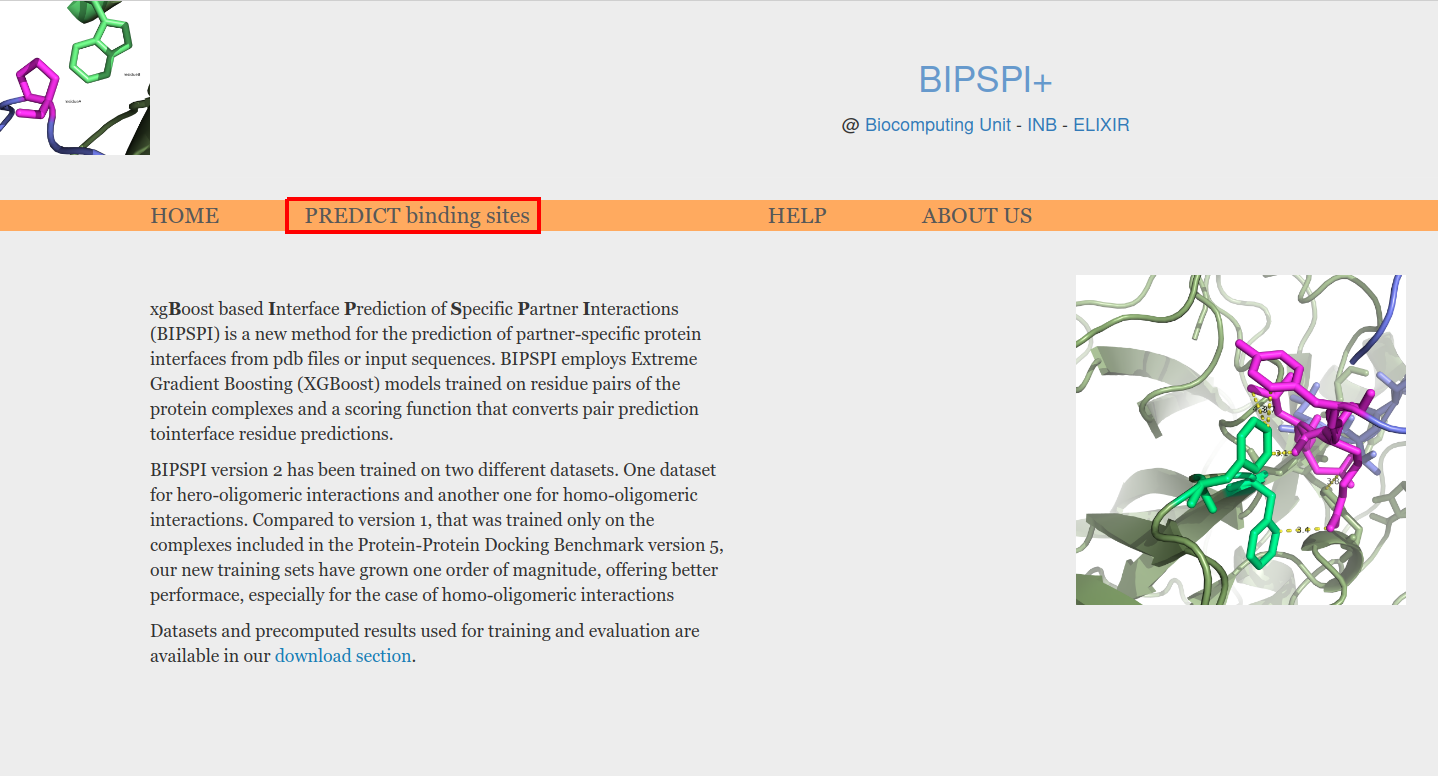
Figure 1. Predictions can be executed under the option "PREDICT binding sites"
"PREDICT binding sites" page allows you to provide the inputs required for BIPSPI.
First, select between homo-complex or hetero-complex prediction (Figure 2, red box). If homo-complex option is selected, only the data corresponding to one protein is required. On the other hand, if hetero-complex option is selected, you will need to provide data for both protein partners.

Figure 2. Select if your protein complex is a homo-complex or a hetero-complex
Prediction for homo-complexes
BIPSPI predictions for homo-complexes can be performed using as input either one atomic model or one sequence. Although BIPSPI has been trained using homodimers only, it is able to provide solutions for other oligomeric posibilities. Yet, better results will be expected predicing homodimers.
Input type can be selected using the radio button (Figure 3.o.1, red box). Available options are atomic model and sequence.
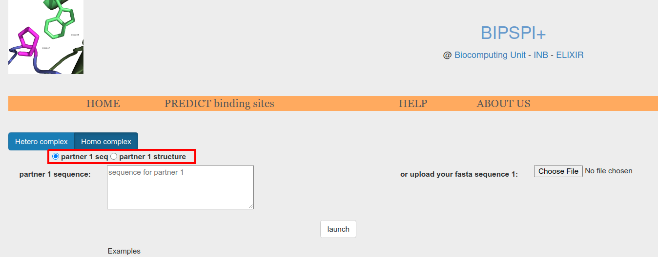
Figure 3.o.1. Input type selector: sequence or atomic model
When sequence input is selected on the radio button (Figure 3.o.1, red box), the sequence can be supplied as plain text in the textbox (Figure 3.o.2, A) or as a fasta file through Choose File button (Figure 3.o.2, B).

Figure 3.o.2. Input form to be used when the input is provided as a sequence
Alternatively, when structure input is selected on the radio button (Figure 3.o.1, red box), the structure can be collected automatically from the Protein Data Bank database (Figure 3.o.3, A) or can be provided as .pdb files through Choose File button (Figure 3.o.3, B). Automatic collection from PDB requires pdb id to be provided (Figure 3.o.3, A.1). Additionally, a particular chain can be specified appending ":ChainId" to the pdb id (e.g. '1ACB:E'). Lastly, a particular biounit can be requiered (Figure 3.o.3, A.2). If not specified or set to 0, asymmetric unit will be collected.

Figure 3.o.3. Input form to be used when the input is provided as an atomic model
Once the input has been provided, computations will start as soon as launch button is pressed.
For a sequence of size 200 amino acids, BIPSPI predictions usually take less than 2 minutes if PSSMs are precomputed in our database or about 10 minutes otherwise. During this time, a waiting page, that is automatically refreshed until results are computed, will be displayed (Figure 4). This page includes the link where results will be available (Figure 4, A), a cancel task buton (Figure 4, B), and the status of the computations (Figure 4, C). Four different status are reported: waiting in queue, computing features, encoding data and computing predictions.

Figure 4. Waiting for predictions
Results page
Three differnt tabs are displayed in Results page: Summary, Residue-Residue Contact Prediction and Partner 1 Interface Residues Prediction.
Summary tab allows for interactive visualization of predicted residues in their sequences (Figure 5.o.1) or their structures (Figure 5.o.2).
A threshold for visualizing the scores can be set using the sliders at the top of the tab (Figure 5.o.1, A or Figure 5.o.2, A). These thresholds are useful to explore different expected precision/recall values. An estimation of the expected precision is used as threshold. Expected precision is computed with an isotonic regression model fitted on the scores pulled across all the benchmark complexes.
When using a sequence as input, it is shown in a sequence box (Figure 5.o.1, B). Sequence index of each amino acid is displayed when mouse is place on its symbol. Amino acids whose score has an expected precision greater or equal than the threshold are highlighted in the sequence box (Figure 5.o.1, B) and also displayed in a table at the bottom of the tab (Figure 5.o.1, C).
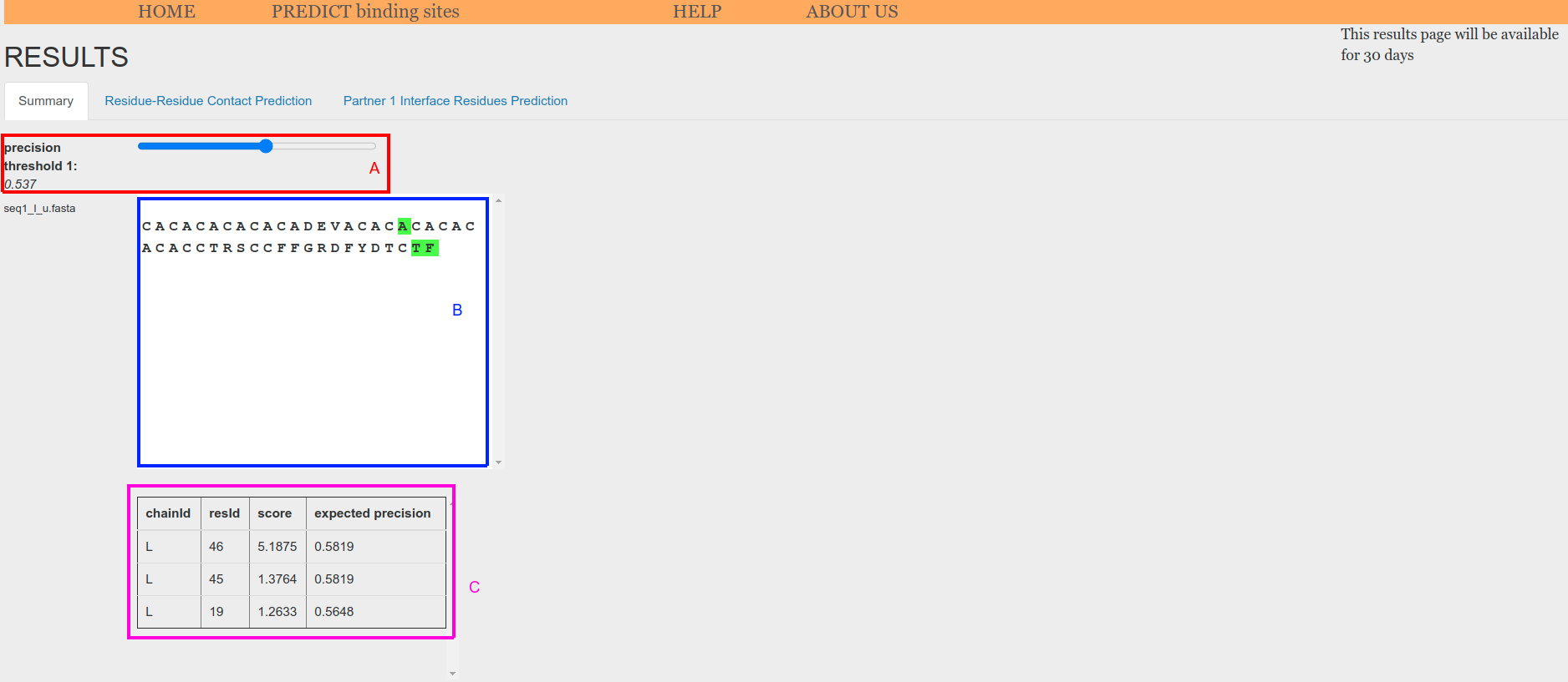
Figure 5.o.1. Prediction from sequence summary
When using an atomic model as input, it is shown in the NGL structural viewers (Figure 5.o.2, B1 and B2). Notice that although only one atomic model is provided as input, the results page displays two copies of it to help visualizing how the two copies may interact and to allow for PatchDock usage. Amino acids whose score has an expected precision greater or equal than the threshold are highlighted in green in the structure (Figure 5.o.2, B1 and B2) and also displayed in tables at the bottom of the tab (Figure 5.o.1, C1 and C2).
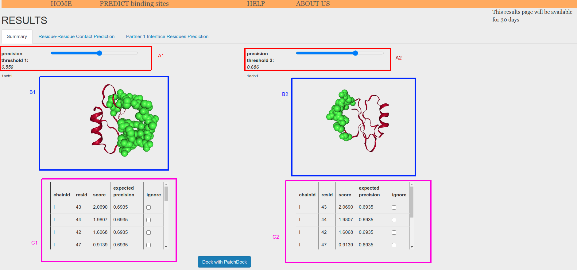
Figure 5.o.2. Prediction from atomic model summary
Residue-Residue Contact Prediction tab (Figure 6) displays a table with the highest score pair predictions and allows for downloading all putative pair predictions. For the homo-oligomer case, when using sequence as input, chainIdL is set to L and chainIdR is set to R despite the fact that both chains are the same. On the contrary, when using an atomic model as input, the original chainId is preserved in both columns. Prediction is an score that goes from 0, no interaction, to 1, very likely interaction.
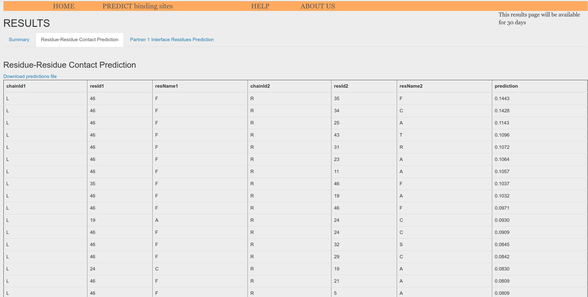
Figure 6. Residue-Residue Contact Prediction table
Partner 1 Interface Residues Prediction tab displays a table with the interface scores predicted for each of the residues of the provided input. The table can be download. The larger the score, the more like the residue belongs to the interface.
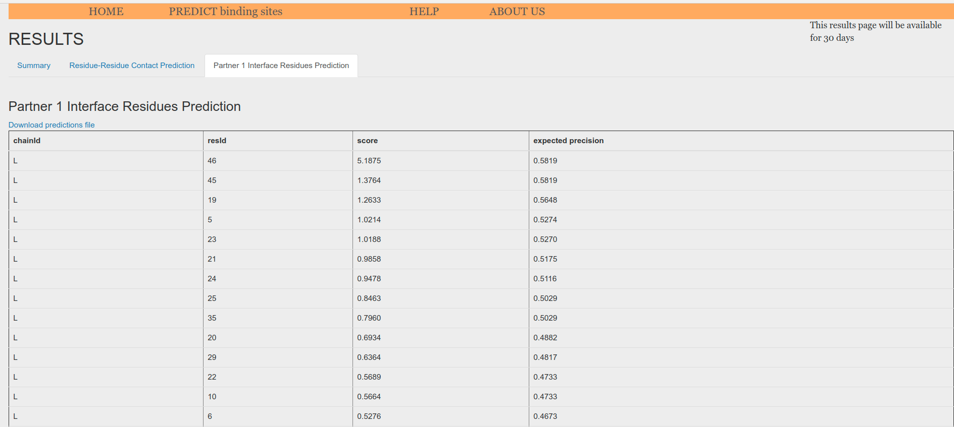
Figure 7. Single Interface Residues Prediction Table
Prediction for hetero-complexes
BIPSPI predictions for hetero-complexes can be performed using as input either two atomic models, two sequences or one atomic model and one sequence. Use the radio buttons for partner 1 (Figure 3.e.1, A) and partner 2 (Figure 3.e.1, A) to select the type of input you will provide.

Figure 3.e.1. Input type selector for each partner: sequence or atomic model
Sequences can be supplied as plain text using textboxes (Figure 3.e.2, A) or as fasta files through Choose File button (Figure 3.e.2, B).
Structures can be collected automatically from Protein Data Bank database (Figure 3.e.2, C) or can be provided as .pdb files through Choose File button (Figure 3.e.2, D). Automatic collection from PDB requires pdb id to be provided (Figure 3.e.2, C1). Additionally, a particular chain can be specified appending ":ChainId" to the pdb id (e.g. '1ACB:E'). Lastly, a particular biounit can be requiered (Figure 3.e.2, C2). If not specified or set to 0, asymmetric unit will be collected.
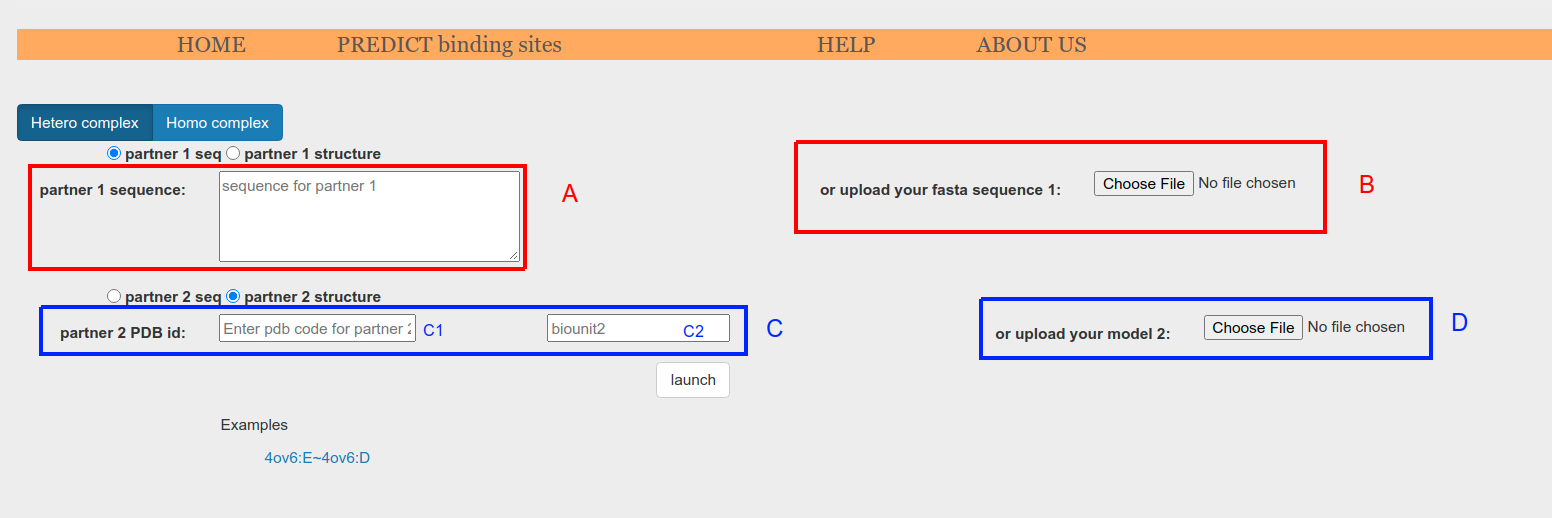
Figure 3.e.2. Input form showing how to provide sequences or structures. Any combination sequence-structure is allowed
Once the input for each partner has been provided, computations will start as soon as launch button is pressed.
For a sequence of size 200 amino acids, BIPSPI predictions usually take less than 2 minutes if PSSMs are precomputed in our database or about 10 minutes otherwise. During this time, a waiting page, that is automatically refreshed until results are computed, will be displayed (Figure 4). This page includes the link where results will be available (Figure 4, A), a cancel task buton (Figure 4, B), and the status of the computations (Figure 4, C). Four different status are reported: waiting in queue, computing features, encoding data and computing predictions.

Figure 4. Waiting for predictions
Results page
Four different tabs are displayed in Results page: Summary, Residue-Residue Contact Prediction, Partner 1 Interface Residues Prediction and Partner 2 Interface Residues Prediction.
Summary tab allows for interactive visualization of the predictions. Depending on the input type, three diferent types of summary tabs are available: sequence vs sequence (Figure 5.e.1), sequence vs structure (Figure 5.e.2) and structure vs structure (Figure 5.e.3).
A threshold for visualizing the scores can be set using the sliders at the top of the tab (Figure 5.e.1-3, A). These thresholds are useful to explore different expected precision/recall values. An estimation of the expected precision is displayed as threshold.
When using two sequences as input, they are shown in two sequence boxes (Figure 5.e.1, B1 and B2). Sequence index of each amino acid is displayed when mouse is place on its symbol. Amino acids whose score has an expected precision greater or equal than the threshold are highlighted in the sequence boxes (Figure 5.o.1, B1 and B2) and also displayed in tables at the bottom of the tab (Figure 5.o.1, C1 and C2).
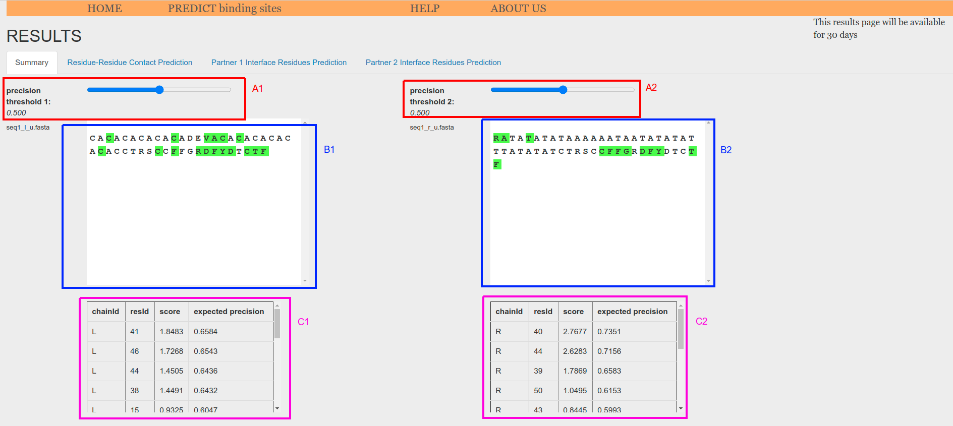
Figure 5.e.1. Prediction from sequence-sequence summary
When using one atomic model and one sequence as input, the atomic model is displayed in the NGL structural viewer (Figure 5.e.2, B2) whereas the sequence is displayed in the sequence box (Figure 5.e.2, B1). Amino acids whose score has an expected precision greater or equal than the threshold are highlighted in green in the structure (Figure 5.e.2, B2) and in the sequence (Figure 5.e.2, B1). Tables showing the highlighted residues and their scores are displayed at the bottom of the tab (Figure 5.e.2, C1 and C2).
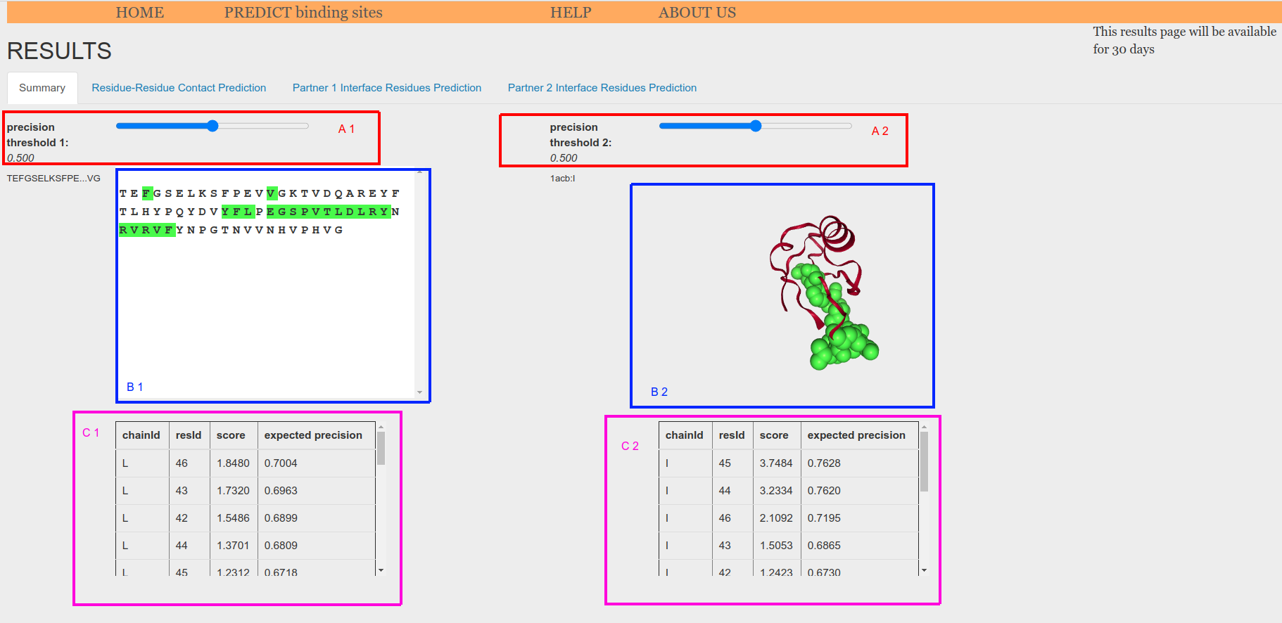
Figure 5.e.2. Prediction from sequence-structure summary
When using two atomic models as input, they are shown in the NGL structural viewers (Figure 5.e.3, B1 and B2), each representing a different interacting parnter. Amino acids whose score has an expected precision greater or equal than the threshold are highlighted in green in the structure (Figure 5.e.3, B1 and B2) and also displayed in tables at the bottom of the tab (Figure 5.e.3, C1 and C2).
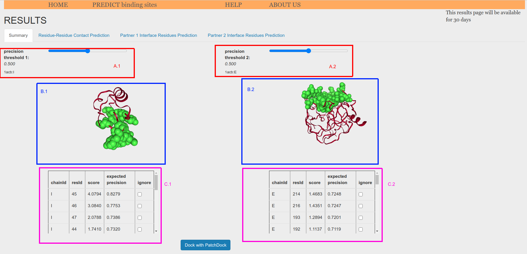
Figure 5.e.3. Prediction from structure-structure summary
Residue-Residue Contact Prediction tab displays a table with the highest score pair predictions and allows for downloading. Prediction is an score that goes from 0, no interaction, to 1, very likely interaction.

Figure 6 Residue-Residue Contact Prediction table
Partner 1 Interface Residues Prediction tab and Partner 2 Interface Residues Prediction tab displays a table with the interface scores predicted for each of the residues of the corresponding partner. The table can be download. The larger the score, the more like the residue belongs to the interface.

Figure 7. Single Interface Residues Prediction Table
PatchDock
PatchDock is a light protein-protein docking algorithm that performs fast rigid body docking. Within this web, you can launch PatchDock using BIPSPI predictions as restrains. To do so, you need first to compute binding site predictions using as input a structure for the homo-complexes case or two structures for the hetero-complexes case.
After that, you will be able to launch PatchDock from the summary tab on Results page (Figure 8). To do so, you first need to fix a threshold for the two protein partners that will define the binding sites to be used as restrains for PatchDock (Figure 8, red boxes). If you want to exclude some of the residues that are above the threshold. you can check the ignore boxes for those residues (Figure 8, blue boxes). This feature is interesting if BIPSPI has produced solutions including several patches and you want to dock each patch independently.
Finally, click on the "Dock with PatchDock" button (Figure 8, magenta box) to launch PatchDock.
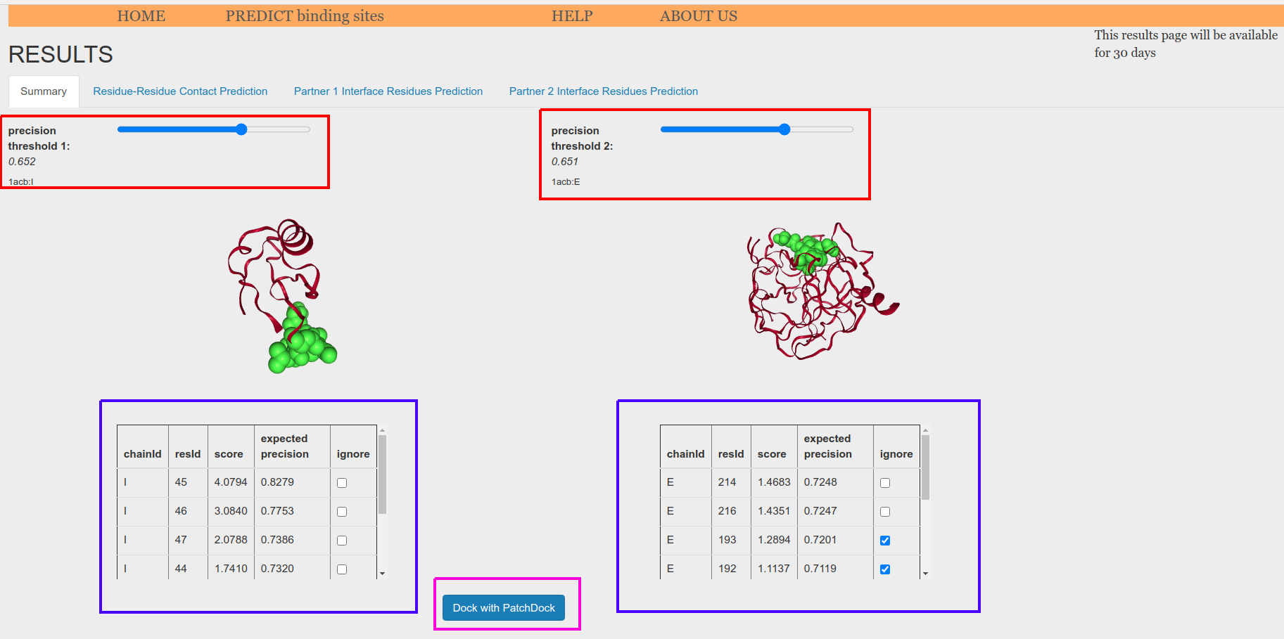
Figure 8. Summary page for binding site prediction using structure(s) as input. This page is used to launch PatchDock
PatchDock solutions will be computed in approximately one minute after the jobs gets out of the queue. A waiting page will be shown while waiting in the queue

Figure 9. Waiting for PatchDock results page
PatchDock results page (Figure 10) will interactively present the top-10 highest score solutions produced by PatchDock. The selector in the top left-hand side corner can be used to navigate between the proposed models (Figure 10, A). The selected solution will be displayed in the NGL structural viewer (Figure 10 B) and the atomic models for the ligand and receptor partners of such solution could be downloaded using the "Download Ligand" and "Download Receptor" buttons (Figure 10, C1 and C2). The model for the receptor is always the same. The scores for the docking solutions computed by PatchDock are reported in a table (Figure 10, D), with the current solution row highlighted in yellow.
Finally, all top-10 highest score solution models together with the transformation file (translation and rotation for all proposed solutions, potentially thousands) generated by PatchDock, can be download through the downloading link "Download all solutions" (Figure 10, E).
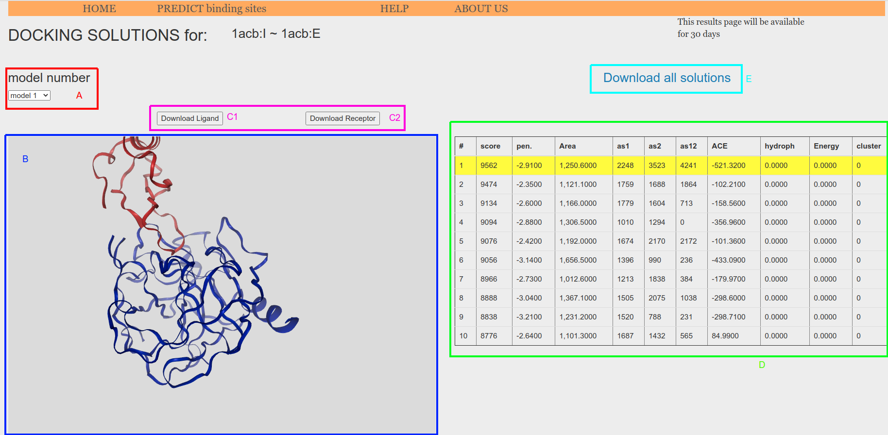
Figure 10. PatchDock results page
